cluscomp output
Cluscomp has very simple output. Basically, for two given partitions of a dataset, it will simply output a single line like this:
Partition1 vs. Partition2 = x.xxx
This is it saying that the two partionings of the dataset are in correspondence
with each other to a degree x.xxx.
As explained in the Manual, cluscomp currently offers two different measurements of partition correspondence: the Hubert-Arabie Object Triple index (which it uses as the default), and the Corrected Rand Index, which is used by specifying the -r option.
Simple datasets
As a simple example, consider the dataset shown here:

This dataset consists of three clusters, one of 34 points, and two of
33 points.
Let's say that you want to test some clustering software you are developing.
As a first run, your software partitions the original dataset nearly correctly,
except for one misclassified point:
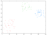
cluscomp will then output:
> cluscomp orig.xml one.xml

        orig vs. one = 0.989699
> cluscomp -r orig.xml one.xml

        orig vs. one = 0.9697
As a second run, your software partitions the original dataset slightly
worse--there are now two misclassified points:

cluscomp will then output indexes of a slightly lower value:
> cluscomp orig.xml two.xml

        orig vs. two = 0.979637
> cluscomp -r orig.xml two.xml

        orig vs. two = 0.940357
The third time you run it, your software partitions the original dataset
pretty badly. It has merged two of the clusters into one:

cluscomp's output will now have very low values:
> cluscomp orig.xml three.xml

        orig vs. three = 1
> cluscomp -r orig.xml two.xml

        orig vs. three = 0.57379
For the sake of illustration, let's say that you try two more times,
and each time, the software misclassified another point:

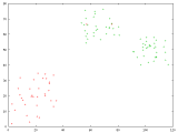
The indexes output by cluscomp will continue to decrease:
> cluscomp orig.xml four.xml

        orig vs. four = 0.970582
> cluscomp -r orig.xml four.xml

        orig vs. four = 0.55902
> cluscomp orig.xml five.xml

        orig vs. five = 0.942965
> cluscomp -r orig.xml five.xml

        orig vs. five = 0.545038
Larger datasets
Here is an example with a larger dataset. In the original set A,
there were 5 clusters, each of 200 "normal" points, and 50 "outlier"
points. That set can be seen here:
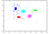
In this graph, each cluster's points (both normal and outlier) are color-coded.
The first attempt at partitioning the raw data produced a dataset B,
which is shown in the next image:
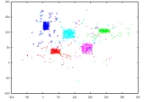
As the color-coding shows, this attempt at partitioning seems very good.
If you look closely however, some of the outlier points have been incorrectly
classified as belonging to the wrong clusters. Cluscomp reflects this:
> cluscomp A.xml B.xml

        A vs. B = 0.964158
> cluscomp -r A.xml B.xml

        A vs. B = 0.850113
The second attempt produced the dataset C, shown here:
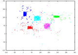
Again, the color-coding shows a very good partitioning, except for a few
misclassified outliers. Cluscomp shows that this attempt was slightly
better then the first:
> cluscomp A.xml C.xml

        A vs. C = 0.970081
> cluscomp -r A.xml C.xml

        A vs. C = 0.871524